CH 2 Neuroscience and ML
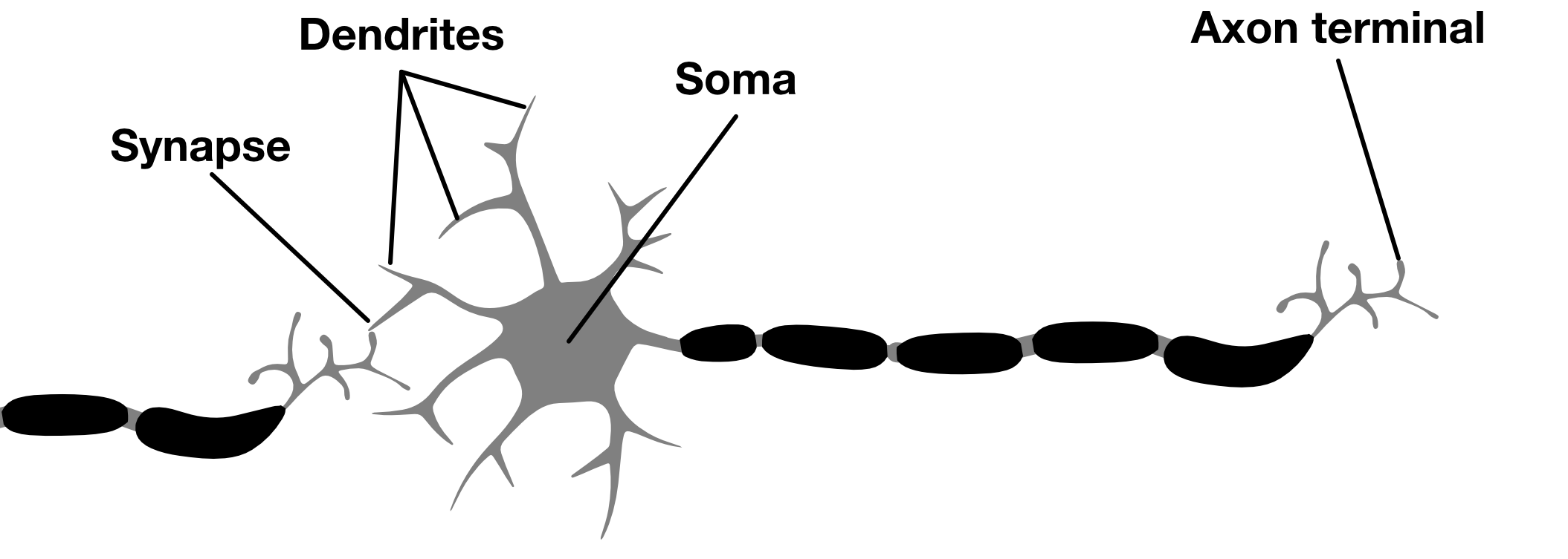
Despite the importance of computers for conducting machine learning and computational neuroscience research both fields had origins long before contemporary transistor computers. In 1943, inspired by the “all-or-none” nature of neural activity, Warren McCulloch (neuroscientist) and Walter Pitts (logician) formalized a simple mathematical definition of a neuron (McCulloch and Pitts 1943). McCulloch and Pitts neurons became the fundamental unit of artificial neural networks (ANN). These artificial neurons, often referred to as (artificial) units, reproduce several key properties of real neurons (Figure 2.1 ). Biological neurons receive input from many other neurons via connections (e.g. synapses) to its dendrites. These synaptic inputs are summated at the soma where the net dendritic input increases or decreases the neurons membrane potential (Fig 2.1). If the net dendritic input shifts the membrane potential beyond a certain threshold (e.g. the threshold potential) the neuron will fire action potentials.

Figure 2.1: Synaptically connected neurons in the brain are the substrate of neural computation in brains
2.1 Artificial Units
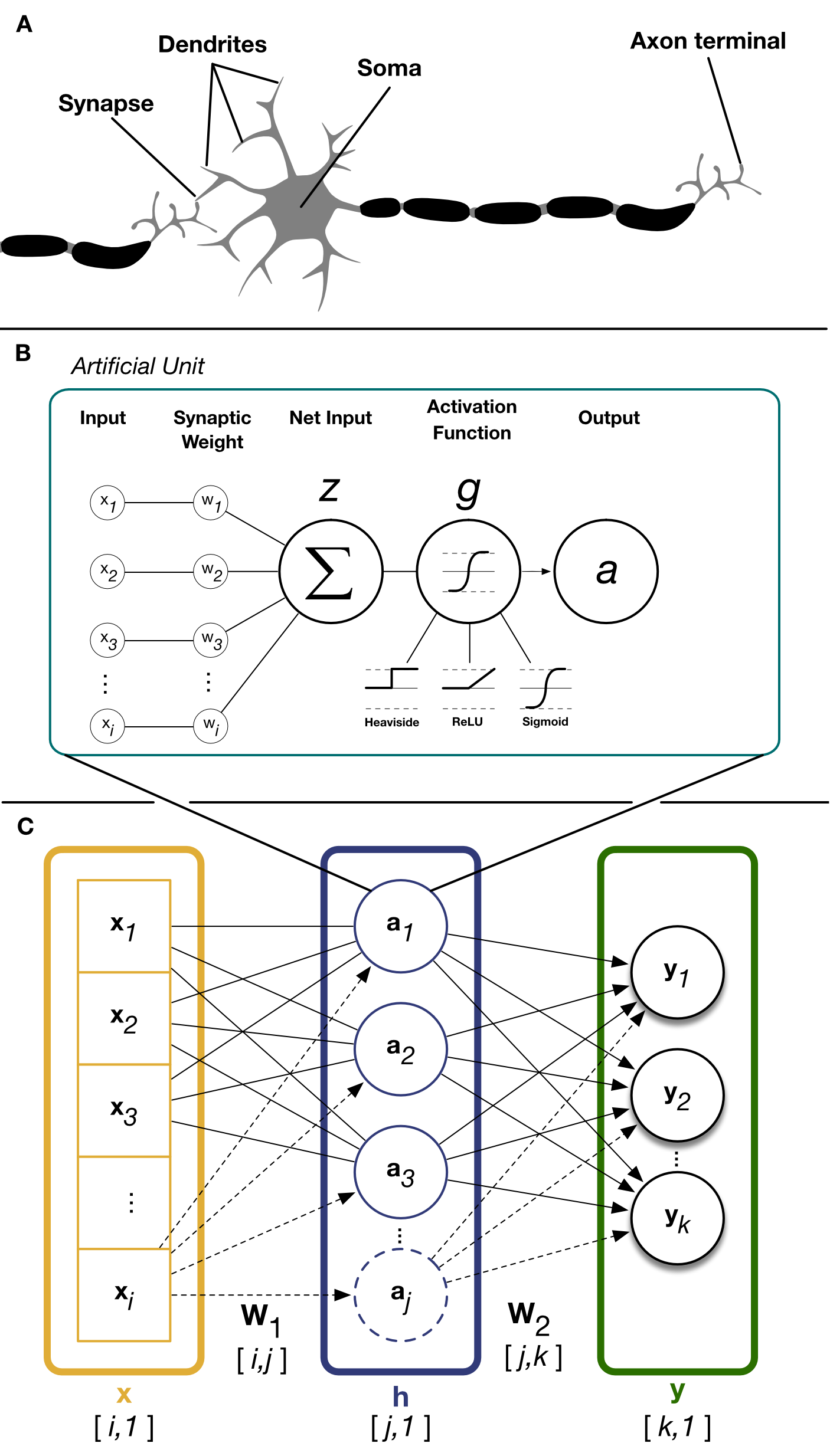
Artificial units (Fig 2.2B) are the basic building block of artificial neural networks. Each artificial unit receives input represented as a sequence of inputs \(x_i\) and each input has a corresponding synaptic weight \(w_i\). The membrane potential \(z\) of the artificial unit is represented by adding net dendritic input to a scalar bias term \(b\) which represents intrinsic excitability. Finally, the threshold non-linear response of biological neurons is captured by passing the units membrane potential \(z\) through an activation function \(g\) which gives the unit output firing rate, or “activation”, \(a\).
\[ \begin{equation} a = g(z) = g(\sum_{i}{w_i x_i}+b) \tag{2.1} \end{equation} \]
2.2 Layers
Just as the brain is comprised of more than one neuron, most models make use of many artificial units. Similar to the laminar organization of the neocortex, artificial neural networks (ANN) group individual units together in layers (Fig 2.2C). The artificial units within a layer collectively operate on a shared input and the layers output consists the collective activations of its constituent artificial units. ANN layers in a model between the inputs (x) and final outputs (y) are often referred to as “hidden” layers. The layers of an ANN are often considered analogous to a population of neurons in regions of the brain which perform similar functions. For instance, primary visual cortex (V1) contain a population of neurons which receive visual inputs from the retina (relayed by LGN). As a population of neurons, V1 processes this visual input and this processed visual information is then relayed to area V2 for subsequent processing.

Figure 2.2: Real neurons and artificial units
2.3 Model Archetypes
Deep artificial neural network models typically have multiples of these layers stacked one after the other, such that the outputs of one layer become the inputs for the subsequent layer. Deep ANN models are often constructed for a specific purpose, or to perform a specific task. Models are often categorized based on purported task and the structure of the inputs it uses to accomplish this task. For instance, many computer vision researchers train models which, given an image, categorize the object in the image.
2.3.1 Classifiers
Classifiers are a class of models that attempt to predict the best category that describes the input from a discrete number of categories. For example, a classic machine learning exercise has been to train a model to predict the category of an object depicted in an image. MNIST, Fashion-MNIST (Xiao, Rasul, and Vollgraf 2017), CIFAR10/100 (Krizhevsky and Hinton 2009) and ImageNet are examples of large labeled image datasets that have been historically popular for evaluating a model’s classification performance. Classifiers are not specific image tasks and can be used on any discrete labeling task. For instance, in Chapter 3 we trained an ANN classifier to predict behavioral sleep state in human PD patients based on features from local field potential spectral decompositions.
2.3.2 Regressors
Regressors use their inputs and attempt to predict a continuous value purportedly derived from the input. Recently, neural network models have been used as functional models of the visual system. These models use images to predict neuronal firing rates observed in animals after viewing the same image and has been used to successfully for predicting stimulus evoked activity in retina (McIntosh et al. 2016) and Inferior Temporal cortex (IT) (Yamins et al. 2014). We successfully utilized a convolutional neural network regressor model to predict firing responses for populations of neurons in macaque primary visual cortex (V1) which is the subject of Chapter 5.
2.3.3 Autoencoders
Autoencoders are a special class of models which attempt to predict their inputs. This is a trivial task if each the intermediate hidden layers have similar dimensionality as the input and output; the model can simply learn to copy the input into the output. Instead, these models are more often configured to have far few dimensions in their hidden layers. In this configuration the only way to successfully perform the task is to exploit information redundancy in the input to compress the input while retaining as much information as possible.
2.4 Layer Architectures
Training an ANN model using machine learning typically requires three components. These components are 1) the model’s layer architecture, 2) objective or loss function, and 3) the models learning rules. The layer architecture of a model explicitly specifies how the artificial units, organized in layers, are connected from input to output. There are a wide variety of layers to choose from when constructing a deep ANN but for the sake of brevity only descriptions of layer architectures used in this work will be provided.
2.4.1 All-to-all
All-to-all layers are the simplest and oldest of layer architectures. In all-to-all layers, every input is connected to every unit in the layer. We can modify the previous equation to describe the entire layer instead of a single unit. Mathematically, we represent the layers input and ouput firing rates as a vector of the individal unit activations \((a_j)\) where each element \(j\) of the vector is a single units activation. By extension, we change the inputs from a scalar to the vector \((x_i)\) where each element \(i\) is an input. Multiplying the input \(x_i\) by the weight matrix \(w_{i,j}\) gives an activation of output of length \(j\):
\[ a_j = g(z_j) = g(x_i \cdot w_{i,j} + b_j) \]
2.5 Loss Function
Loss or cost functions ( \(J\) ) are mathematical definitions of the goal of the learning system. The loss function is used to calculate a scalar metric quantifying the models’ task performance as a function of its output. Loss functions can take any form mathematically as long as they are 1) differentiable and 2) convex. Reconstruction error (sum of squared pixel errors) were traditionally used for training models which attempt to generate a particular image. We can express the sum squared pixel loss between an image \(\hat{y}\) and the target reference \(y\) as:
\[ J(y,\hat{y}) = \sum (y-\hat{y})^2 \]
Objective functions don’t have to depend on a particular dataset or task. For instance, sparse coding models use activation sparseness and reconstruction error as their objective function to learn sparse representations. When minimized over images of natural scenes they learn a set of basis functions that resemble localized receptive fields of simple cells in primary visual cortex (Olshausen and Field 1996)
2.6 Learning Rules
Once a model’s architecture and objective function are specified “training” it is simply optimizing the parameters of each layer to improve its loss. The algorithm for how to iteratively update the ANN model parameters to minimize loss was first demonstrated by Rumelhart (Rumelhart, Hinton, and Williams 1986) and it is a simple 2 step process:
- Forward pass: Use a batch of \(x\) input values to calculate the predicted outputs \(\hat{y}\)
- Backpropogation: Use prediction error to update weights and biases
To illustrate this process, we will derive it for a simple 2-layer ANN. For simplicity, we change notation when describing deep ANN with multiple layers such that variable and function subscripts denote the variable or function’s corresponding layer NOT matrix or vector dimensions. For instance, we define the output activations of the lth layer in a model comprised of sequentially stacked all-to-all layers as:
\[ a_l = g(a_{l-1} \cdot W_l + b_l) \]
2.6.1 Forward Pass
First, we pass a batch of training example inputs (\(x\)) through the model to get a batch of output classifications (\(\hat{y}\)). Given our simple feedforward layer defined above, the full equation for the models output is given by:
\[ \hat{y} = g(W_2 \cdot g(W_1 \cdot x +b_1) + b_2) \]
Our loss function \(J\) defines how to evaluate the model’s performance as a function of the model’s predicted and target values. The target value is also sometimes referred to as the teaching signal, as it’s used to teach the model the correct output for a given input. For this example, we’ll use sum-squared-error:
\[ J(y,\hat{y}) = \sum (y-\hat{y})^2 \]
2.6.2 Backpropagation
To derive the gradient of the loss function with respect to the model parameters (\(\nabla_{\theta} J\)) we take a partial derivative of the objective function with respect to the models parameters:
\[ \nabla_{\theta} J = \frac{\partial J(\theta ; y, \hat{y})}{\partial \theta} \]
2.7 Optimizers
Once we know the gradient of each weight with respect to the loss, we simply need to adjust the weights of the model in the direction specified by the weight gradient. Continually descending the gradient of the loss function should theoretically result in the optimal weights for performing the model’s task.
2.8 Summary
The purpose of this chapter is not to exhaustively cover the field of machine learning but instead to serve as a brief primer of concepts and terms you will encounter in subsequent chapters. Chapter 2 uses an ANN classifier comprised of fully-connected layers to predict sleep states from LFP spectral decompositions. Chapter 3 utilizes a convolutional autoencoder/classifier hybrid model to test hypotheses about computational objectives employed in primate ventral stream visual representations. Finally, Chapter 4 uses a convolutional neural network (CNN) to directly regress neuronal activity in macaque primary visual cortex. Hopefully, you can appreciate the similarities between artificial neural networks and the biological neural networks that inspired them. If nothing else, remember that using machine learning to train ANN models hinges on three components:
- Model architecture
- Loss function
- Learning rules
All three components influence both transient and final model performance.